Goal

Ethereum introduced EIP 1559 which brought many changes to how ethereum worked. One of the big changes was that transactions included a basefee. Since there were already assumptions about how basefee might behave, simulations could be created and compared to actual basefee behavior to try and verify if the original assumptions were correct. Interestingly enough, aside from verifying assumptions, many other discoveries were found in the simulation analysis.

Assumptions

• Variables that we wanted to model were valuation and gas used
• Miners accept highest bids first
• Base follows the following update function which will be explained later:

Valuations

Definition: Valuations is an economic term which means how much a good is worth to a person.

In the most simple scenario, this means a valuation can be found by how much a person is willing to pay for a good. However, the data team I worked with was also interested in how valuations change both pre- and post-EIP 1559. So simply using the highest bid would not be sufficient in this case.

Solution: In order to try and tease out a users valuation, we took their bids and divided it by a common reccommended bid provided by Go Ethereum (GETH). Most users of Ethereum will see the GETH recommended bid as they are putting in their transactions so how they bid relative to GETH recommendation is a good indicator of their valuation. Mathmatically, we defined valuations as (user’s bid)/(GETH recommended bid).

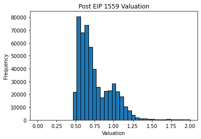
Above is a histogram showing valuations generated by using bids from October 2021. There are two interesting points here:

• There is a lot of white space on the left. This is because the histogram only includes transactions which were included into the blockchain. There must be some cut off point at which a user does not bid high enough to get included into the blockchain and this happens to be at around 0.5 of GETH recommended bid.
• It looks like there are two distributions, one centered roughly around 0.6 and one centered roughly around 1.0. I considered this to be evidence that there are two types of users, low and high valuation users. Around 66% of the users were of low valuation and around 33% of the users were of high valuation.

Disclaimer: When modelling valuations, I used a Gamma distribution, this was to help other members of my team that needed a named distribtuion for valuations. This is not neccesarily the best distribution to fit to valuations, it is more likely that a non-parametric model may be a better fit.

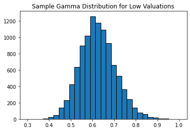
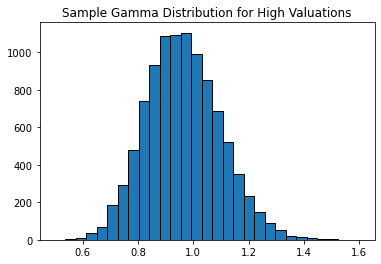
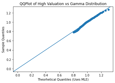
Above are the histograms of gamma distributions that were fitted to the valuation and the QQ plots of the gamma distributions. The QQ plots aren’t quite a perfect fit but they are pretty close. The parameters of the low valuation gamma distribution are k=59.6849 and theta=0.0105. The parameters of the high valuation gamma distribution are k=52.1001 and theta=0.0185. The parameters were solved for by using maximum likelihood estimator.

Gas Used

Definition: Gas is how complex a transaction is to be included into a blockchain. While not strictly true, it is a good proxy as a metric for demand.

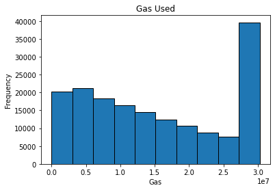
Above is a histogram of how much gas is used per transaction. Notably, it doesn’t really look like any named distribution but that’s ok. In this case, I simply bootstrapped the gas used in order to use it in the simulation.

Base Fee Update

As mentioned earlier, the base fee update formula is:

• b=base fee
• d=learning rate
• g=gas used What the formula is saying is that the next base fee will increase or decrease if gas used is higher or lower than target gas used respectively. Simply, if demand increases then base fee increases. Target gas used is 15 million which was set by Ethereum. D is the learning rate, this is to help prevent sudden spikes in base fee.

Simulation

This will be a very brief summary of how the simulations work, the finer details can be found in the code. Basically, now that I have a model for how full blocks will be and how much users will bid for their transactions, I can simulate blocks and fill them with transactions. This also means that I can simulate how the base fee behaves.

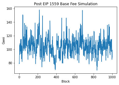
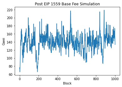
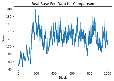
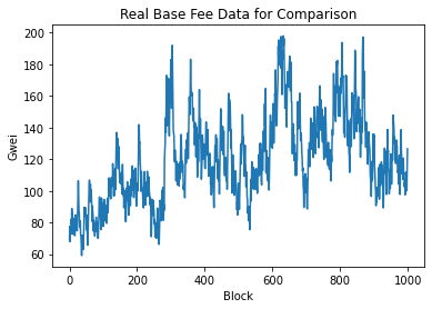
So the simulation looks somewhat similar to real base fee. One interesting property is that the spikes going upward tend to be really sharp and take only a couple of blocks while spikes going downwards are fatter and takes more blocks to occur. Finally, I use an ARIMA model to compare the two time series.

ARIMA

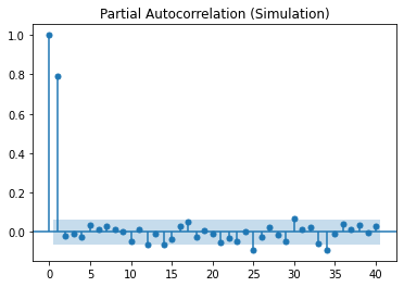
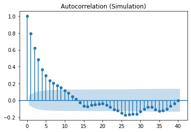
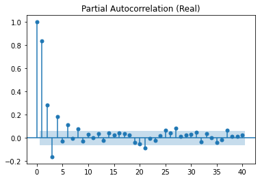
Below are the PCAF and ACF graphs which suggest parameters of p=2, d=0 and q=0.

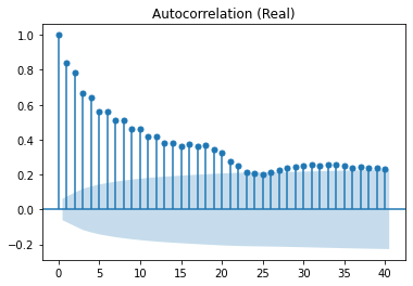
Then below are the graphs of the residuals:

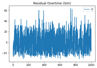
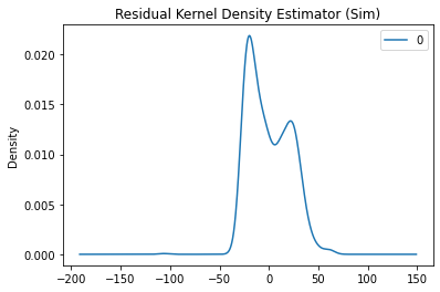
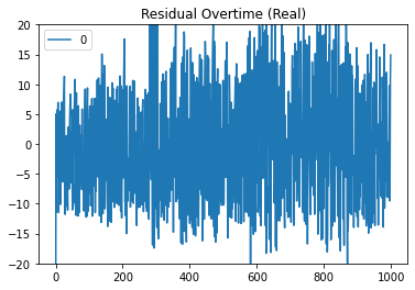
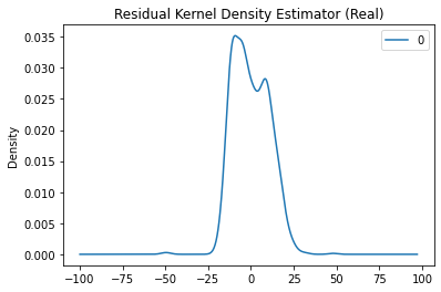
So it looks like the ARIMA models aren’t fitted perfectly to the time series but an interesting note is that the ARIMA models tend to underpredict the base fee more often than overpredict. This is likely due to the sudden sharp spikes which I think is caused by the idea that there are two distributions of users, low and high valuation users. In the simulation formula, inclusion of high valuation users always increases the base fee whereas low valuation users do not neccesarily decrease the base fee.

Conclusion

Overall, improvements can be made to the simulation but it was able to generate ARIMA models with similar parameters to the ARIMA model for real base fee data. Going forward, I think the main way to improve this simulation is if there was a variable to distinguish low valuation and high valuation users.