Goal:

The goal of this project is to benchmark machine learning techniques when used to classify sound files.

Supervised Machine Learning Techniques used:

• Gaussian Naive Bayes
• Decision Trees
• K Nearest Neighbors

Unsupervised Machine Learning Techniques used:

• K Means

  Dataset

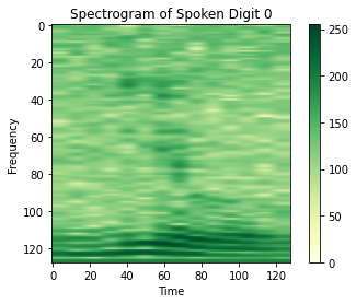
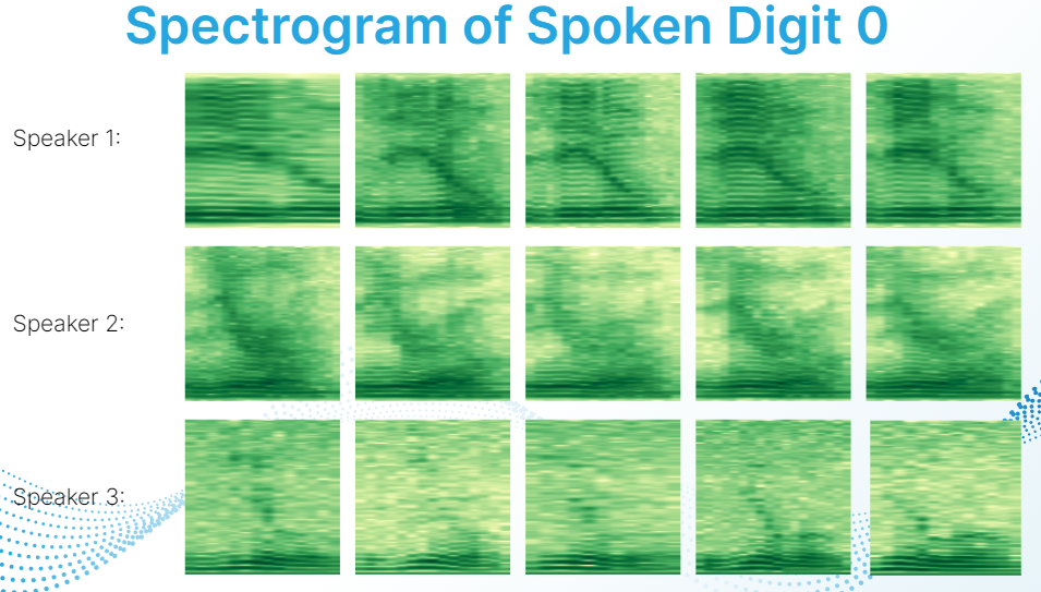
The dataset used can be found in the repository and is called MNIST_Spoken_Digits.rar. This dataset contains spoken digits from 0 to 9. There are 3000 .wav files in the dataset and each individual spoken digit has 300 .wav files. There are 6 different speakers who generated these .wav files. Each sound file is transformed into a spectrogram prior to classification so this project uses image recognition techniques to try and classify sounds.

• Sample Spectrogram:

Benchmarking

Cross validation combined with confusion matrices were the main benchmarks. K means has it’s own way of benchmarking since it is an unsupervised technique and will be discussed later.

Cross Validation:

10-fold cross validation was used in each test. This means that each dataset was randomly divided into 10 subsets and 10 tests were used. In each test, one of the subsets would be considered as test data while the remaining 9 subsets would be considered as training data.

Confusion Matrix:

The confusion matrix serves as a visual to see how well each machine learning technique performed. In my confusion matrices, the predicted labels are along the x-axis while the true labels are along the y-axis. Any number that is not along the diagonal of the matrix represents incorrect classifications. (Note: There are 10 different tests so the confusion matrices being shown are a sum total of all 10 confusion matrices.)

Gaussian Naive Bayes:

• How it works:

Gaussian Naive Bayes is a model based supervised machine learning technique. It assumes that each class (or each of the spoken digits from 0 to 9) can be approximated by a Gaussian distribution (or equivalently, normal distribution). The training data is used to get the maximum likelihood estimators (MLE) for the parameters of each Gaussian distribution for each class.

• Result:

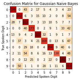
Overall Accuracy: 65.59%

• Deeper Analysis:

• Conclusion:
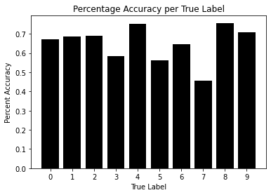
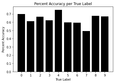
  Overall, Gaussian Naive Bayes performed poorly. It has an overall accuracy of 65.59% which is a little better than pure random guessing.

  • The accuracy can be further analyzed by looking at the accuracy given a true label and the accuracy give a predicted label. Given any true label, the accuracy fluctuates between 46% and 77%. This isn’t very impressive as it suggests for digits like 3,5 and 7 the model is just purely guessing and even for it’s best digit (spoken digit 8) it only does ok at best.
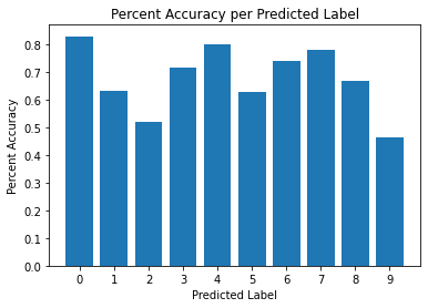
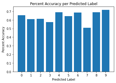
  • A similar analysis can be done given that the model has predicted a spoken digit. Given any predicted label the accuracy fluctuates between 46% and 82%. This is also a poor result. Given that the model predicts a digit like 2,5 or 9, it is as good as a random guess. Given digits like 0,4 or 6 the model performs ok at best.
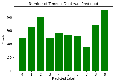
  • This particular model overpredicts 9 as the spoken digit. Within the code are tests using this model without the spoken digit 9 but since the results did not improve much, they were not added to this document.

Decision Tree:

• How it works:

Decision Trees try to classify data points by separating each data point by their features (or equivalently the columns in this case). Generally, decision trees perform better when the features are highly correlated to the class that is being predicted. This means that decision trees generally do not perform well for image recognition such as our tests with spectrograms. Each pixel of the spectrogram is a feature in this case but each pixel also contains very little information about the classification of the overall data point.

Even though the results are expected to be poor, the goal of this project is to benchmark each technique. This particular experiment is to verify the expected result.

• Result:

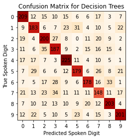
Overall Accuracy: 63.76%

• Deeper Analysis:

• Conclusion:
  Overall, decision trees performed poorly when trying to classify spectrograms. It has an even lower overall accuracy of 63.76% which is slightly better than guessing. Furthermore, when looking at the deeper analysis, the individaul accuracies are very poor as well.
  • The accuracy per true label fluctuates between 49.33% and 75%. While this looks similar to Naive Gaussian Bayes, it may actually be worse. Most true labels hover around a 60% accuracy which means given any true label the model is mostly just guessing. Compared to Naive Gaussian Bayes, even though it wasn’t performing well with every true label, it did perform well with some.
  • The accuracy per predicted label fluctuates between 51.03% and 71.79%. Similar to percent accuracy per true label, the percent accuracy per predicted label seems to be consistently low and most predicted labels hover around 60% accuracy.
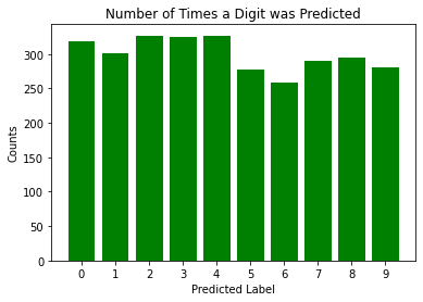
  • No number was overpredicted with decision trees unlike in Naive Gaussian Bayes. It looks like most digits were predicted at roughly the same frequency which is good. This is the only aspect in which decision trees seemed to work well, no individual digit dominated or was under-represented.

K Nearest Neighbors

• Result:

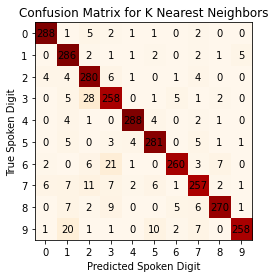
Overall Accuracy: 90.86%

• Deeper Analysis:

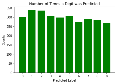
• Conclusion:
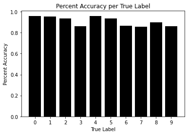
  Easily the best performing technique so far with an accuracy of 90.86%. Still far from ideal but it is something that can be further worked upon. Also, the graphs from the deeper analysis don’t show any glaring flaws either.
  • The percent accuracy per true label ranges from 85.67% to 96%. The lowest accuracy is 85.67% which isn’t great but isn’t bad either. The true labels this model struggles the most with are 3,6,7 and 9.
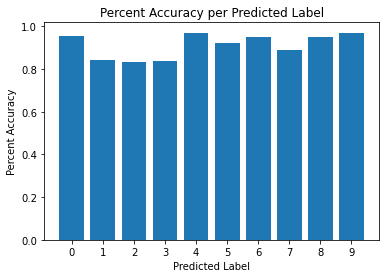
  • The percent accuracy per predicted label ranges from 83.33% to 96.99%. As before, the lowest accuracy is 83.33% which isn’t great but isn’t terrible either. The predicted labels with the lowest accuracies are 1,2 and 3.
  • There is no obvious dominating or under-represented digit in prediction frequency. Each digit was predicted roughly the same number of times which is what the model should predict.

K Means

• How it works:
  K Means doesn’t use any labels. Instead, it tries to create clusters by minimizing the variance within each cluster. The algorithm is an iterative one in which data points are assigned to the cluster which has the closest mean and then the means are updated by the data points which are assigned to that cluster. Initial starting points are random. (Usually random data points, but the updated means do not need to be an actual data point.)

• Benchmarking:
  Since K Means is an unsupervised technique, the benchmarking will be different and albeit a bit simpler. There are no true labels in an unsupervised machine learning technique so the only way to see how well it performs is if each cluster produced looks like what would be expected. In this case, there should be 10 clusters with 300 data points in each cluster.

K Means was mostly included for curiosity as there is no direct way to compare it with the other supervised machine learning techniques.

• Result:

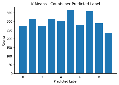
• Conclusion:
  On average, each cluster size is 45.6 off of 300. Looking at the graph though, each cluster looks like they are too far from 300 to consider K Means to be a good method for clustering spectrograms.

Conclusion

• Overall, K nearest neighbors performed the best with an overall accuracy of 90.86%. Further inspection of the spectrograms suggests that this may be because the spectrograms of voices of individuals are similar to each other.

This doesn’t nullify the findings but it does suggest that K nearest neighbors performs well at recognizing a person’s voice as opposed to recognizing a spoken digit. Further research will be needed to see if this is true or not.

• Naive Gaussian Bayes performed second best with an overall accuracy of 65.59%. The results per digit seems to fluctuate with certain digits having a high prediction accuracy while other digits had low prediction accuracy. An interesting thing to note was that digits that were overpredicted tend to have lower prediction accuracy. This may suggest that certain Gaussian distributions for certain digits were simply too large.

• Decision Trees performed the worse with an overall accuracy of 63.76%. This was expected since decision trees expect the features of the data set to have a high correlation to the output but the features of each spectrogram are simply pixels which carry little information and little correlation to the output. No matter how the results are analyzed, most accuracies hover around 60% which suggests that decision trees perform a little better than random guessing.

• K Means was included for curiosity but cannot be directly compared to the other 3 techniques.